Reinforcement Learning – Limit Infinite

Markov Decision Process
Bellman Equation
Dynamic Programming
Model-free Prediction
Model-free Control
Value Function Approximation
Policy gradients
Actor-critic methods

In the reinforcement learning set up, we have a system with states and dynamics among states. Dynamics consist of probabilities for transitions among states and rewards for states. And, there is an agent who can take one of several possible actions in each state. The goal is for the agent to act at each point of time in such a way as to maximize cumulative reward.

Reinforcement Learning is mathematically modeled by a Markov Decision process (MDP).

Markov Decision Process

An MDP is formalized as a tuple $(S, A, P, R, \gamma)$ , where

$S$ : set of states
$A$ : set of actions that can be taken on states
$P$ : a set of matrices where each matrix gives probabilities of transitions from one state to another (Markov property implies current state is good enough to indicate probability of transition to a subsequent state). Rather than one matrix, we need a set of matrices because probabilities of state transitions are dependent on actions taken on the states. So, each matrix in the set is indexed by an action. Thus, an element of a matrix for action $a$ , denoted $P^a_{ss'}$ , is the probability of transitioning to state $s'$ , when action $a$ is taken in state $s$ .
$R$ : This is a set of vectors of rewards(or, precisely, expectation of reward). Each vector gives reward out of a particular state. Thus, an element of vector for state $s$ , denoted by $R^a_s$ is the reward that is given for taking action $a$ in state $s$ .
$\gamma$ : This is the discount factor that is multiplied to future rewards to determine the value of current state or an action in current state.

Goal of an MDP is to determine a decision policy $\pi$ which gives the optimal action to be taken in each given state so that eventually, you accumulate the maximum possible reward. We model $\pi$ as a probability distribution denoted $\pi(a|s)$ to indicate the probability that the agent will take action $a$ in state $s$ .

A state-value function $v_{\pi}(s)$ and an action-value function $q_{\pi}(s, a)$ are defined. $v_{\pi}(s)$ is the total expected reward considering all future possible using the policy $\pi$ from the state $s$ . That is, starting from state $s$ , if we take the current and future actions according to policy $\pi$ , $v_{\pi}(s)$ is the reward that we expect to accumulate given the dynamics ( $P, R$ ) of the system. Likewise, $q_{\pi}(s,a)$ is the total expected reward considering all future possible using the policy $\pi$ from the state $s$ by taking action $a$ now.

Bellman Equation

$v_{\pi}(s)$ and $q_{\pi}(s,a)$ satisfy the Bellman equations as follows:

$\begin{aligned}v_{\pi}(s) &= \sum\limits_a \pi(a|s)\left[R_s^a+\gamma\sum\limits_{s'} P^a_{ss'}v_{\pi}(s')\right] \\ q_{\pi}(s,a) &= R_s^a+\gamma\sum\limits_{s'} P^a_{ss'}\left[\sum\limits_{a'}\pi(a'|s')q_{\pi}(s',a')\right]\end{aligned}$

$v_{\pi}(s)$ and $q_{\pi}(s,a)$ are related to each other as:

$v_{\pi}(s) = \sum\limits_{a}\pi(a|s)q_{\pi}(s,a)$ (Average of $q_{\pi}(s,a)$ over all actions $a$ )

$q_{\pi}(s,a) = R_s^a + \gamma \sum\limits_{s'}P^a_{ss'}v_{\pi}(s')$

In matrix-vector form, we can write:

$V_{\pi} = R^{\pi} + \gamma P^{\pi} V_{\pi}$

Here,

$V_{\pi}$ : a column vector indexed by state $s$ . Each element of $V_{\pi}$ is $v_{\pi}(s)$ .
$R^{\pi}$ : a column vector, where each element is $\sum\limits_a \pi(a|s)R_s^a$ .
$P^{\pi}$ : a square matrix where rows and columns are indexed by states. An element of $P^{\pi}$ is $P^{\pi}_{ss'} = \sum\limits_a \pi(a|s)P_{ss'}^a$ .

Optimal value functions/optimal policy

Optimal state-value function $v_*(s)$ is maximum state-value function over all policies: $v_*(s) = \max\limits_{\pi} v_{\pi}(s)$ .

Optimal action-value function $q_*(s,a)$ is maximum action-value function over all policies: $q_*(s,a) = \max\limits_{\pi} q_{\pi}(s,a)$ .

Theorem: A policy $\pi_*$ called optimal policy exists that achieves optimal state-value function and optimal action-value function.

That is, $v_{\pi_*}(s) = v_*(s)$ for all $s\in S$ , and $q_{\pi_*}(s,a) = q_*(s,a)$ for all $s\in S$ and $a\in A$ .

There could be multiple optimal policies for a system. But, all of them achieve $v_*$ and $q_*$ .

Bellman Optimality equation

Given optimal state-value and action-value functions, we can have a particular deterministic optimal policy $\pi_*$ where:

$\pi_*(a|s) = \begin{cases} 1 & \mbox{ if } a = arg\max\limits_{a'} q_*(s,a') \\ 0 & \mbox{ otherwise }\end{cases}$

For this particular optimal policy, the following equation holds:

$v_{\pi_*}(s) = \max\limits_a q_{\pi_*}(s,a)$ .

This is called the Bellman optimality equation.

Note that, while the regular Bellman equation holds for any policy $\pi$ , the Bellman optimality equation (in addition to the regular Bellman equation) holds for this particular deterministic optimal policy. In fact, it is easy to derive the Bellman optimality equation from the Bellman equation given the probability distribution of this particular $\pi_*$ .

Now, as given by the theorem in previous section, since $v_{\pi_*}(s) = v_*(s)$ and $q_{\pi_*}(s,a) = q_*(s,a)$ , we can drop the $\pi$ from the Bellman optimality equation and have:

$v_*(s) = \max\limits_a q_*(s,a)$

Thus, Bellman optimality equation is an equation for optimal value functions.

Equivalently, Bellman optimality equation is also:

$v_*(s) = \max\limits_a\left[R^a_s + \gamma\sum\limits_{s'}P^a_{ss'}v_*(s')\right]$

And, $q_*(s,a) = R^a_s + \gamma\sum\limits_{s'}P^a_{ss'}v_*(s') = R^a_s + \gamma\sum\limits_{s'}P^a_{ss'}\left[\max\limits_{a'} q_*(s',a')\right]$

The difference between the Bellman equation and the Bellman optimality equation is that the average factor $\sum\limits_a \pi(a|s)$ is replaced by $\max\limits_a$ .

Dynamic Programming

Two techniques from Dynamic Programming may be employed to figure out the optimal policy in the reinforcement learning set up.

The first one is called the policy iteration, while the second one is called value iteration.

Policy Iteration

Here, we start with an arbitrary policy $\pi_0$ . Say, the policy has uniform distribution – that is, we choose all actions with equal probability. For this policy, we initialize the state-value function for all states to an arbitrary value ,say $0$ .

We then iterate through the Bellman equation as follows:

$v^{k+1}_{\pi_0}(s) = \sum\limits_a\pi_0(a|s)\left[R_s^a + \gamma\sum\limits_{s^1}P^a_{ss'}v^k_{\pi_0}(s)\right]$

Or, matrix-vector form:

$V^{k+1}_{\pi_0} = R^{\pi_0} + \gamma P^{\pi_0}V^k_{\pi_0}$

Here, $k$ is the iteration to refine the values of $v_{\pi_0}(s)$ . If we initialized, $v_{\pi_0}(s)$ to $0$ , then we have $v_{\pi_0}^0(s) = 0$ for all $s$ .

When we iterate over $k$ , we will have $v^k_{\pi_0}(s)\to v_{\pi_0}(s)$ as $k\to \infty$ .

Once we thus obtain $v_{\pi_0}(s)$ and $q_{\pi_0}(s,a)$ , we devise a new policy $\pi_1$ that acts greedy on $q_{\pi_0}(s,a)$ . That is, $\pi_1$ is such that:

$\pi_1(a|s) = \begin{cases} 1 & \mbox{ if } a = arg\max\limits_{a'} q_{\pi_0}(s,a') \\ 0 & \mbox{ otherwise }\end{cases}$

Then again, we determine iteratively $v_{\pi_1}(s)$ using the Bellman equation procedure above.

We continue this process iteratively of obtaining a new policy $\pi_n$ and evaluating its state-value function $v_{\pi_n}(s)$ , until the policies (their state value functions??) converge. The resultant policy will be (is deemed??) the optimal policy.

Value Iteration

In this method, we iterate directly using the Bellman optimality equation:

$v_*(s) = \max\limits_a\left[R_s^a + \gamma\sum\limits_{s'}P^a_{ss'}v_*(s')\right]$ .

We again arbitrarily initialize $v_*(s)$ , say, to $0$ , and then use

$v_*^{k+1}(s) = \max\limits_a\left[R_s^a + \gamma\sum\limits_{s'}P^a_{ss'}v_*^k(s')\right]$

iteratively to derive new values of $v_*(s)$ .

Eventually, the process converges. That is, as $k\to \infty$ , we will have $v_*^k(s) \to v_*(s)$ .

Model-free prediction

Dynamic programming enables us to determine the state-value and action-value functions given the dynamics (model) of the system. It does this by mathematically using the Bellman equations and plugging in the dynamics (rewards and probabilities).

If the model (rewards and probabilities) of the system is not known a priori, we can empirically estimate the value functions for a given policy. We do this by taking actions according to the given policy, and taking note of the state transitions and rewards. By making enough number of trials, we are able to converge to the value functions for the given policy.

Monte-Carlo learning

This applies to experiments which are run as episodes. Each episode terminates and next episode is independent of the current episode. As an example, when a board game is played, each new game constitutes a separate episode.

Given a policy, action is taken in each state according to the policy. For a state $s$ that is arrived at time $t$ , return for a particular run through the termination of the episode is calculated:

$G_t = R_{t+1} + \gamma R_{t+2} + \gamma^2 R_{t+3} + \cdots + \gamma^{T-1}R_{t+T}$

Here, $R_t$ is the reward obtained by taking action in the state at time $t$ .

Such returns $G_t$ are added for all the episodes during which the state is visited to obtain total return for the state:

$S(s) \leftarrow S(s) + G_t$

And, number of episodes (or in an alternate method, number of visits??) $N(s)$ that the state is visited is calculated.

Value of the state is estimated as mean return $V(s) = \frac{S(s)}{N(s)}$ , since by law of large numbers $V(s)\rightarrow V_{\pi}(s)$ as $N(s)\rightarrow \infty$ .

Note that running average return can calculated online (real-time) as the episodes are run instead of calculating it only after all episodes are completed as follows:

$V(S_t) \leftarrow V(S_t) + \frac{1}{N(S_t)}(G_t - V(S_t))$

Or equivalently,

$V(S_t) \leftarrow \left(1 - \frac{1}{N(S_t)}\right)V(S_t) + \frac{1}{N(S_t)}G_t$

In practice in online learning scenario, rather than using $\frac{1}{N(S_t)}$ for weighing the return $G_t$ from current episode, a constant factor $\alpha$ with $0 < \alpha < 1$ is used. This leads to the formulation:

$V(S_t) \leftarrow (1 - \alpha)V(S_t) + \alpha G_t = V(S_t) + \alpha(G_t - V(S_t))$

What is the reasoning? Rather than the average over all episodes, returns from recent episodes is given more weight than returns from old episodes. Returns from episodes are given weights that exponentially decrease with time.

Temporal-Difference (TD) learning

In contrast to Monte-Carlo learning, Temporal-Difference (TD) learning can learn the value function for non-episodic experiments.

In Monte-Carlo learning, we run through a complete episode, note the “real” return obtained through the end of the episode and accumulate these real returns to estimate the value of a state.

In TD learning, we do as follows:

we initialize the value for each state.
we run the experiment (according to the given policy) for a certain number of steps (not necessarily to the end of the episode or experiment). The number of steps $n$ we run the experiment is identified as $n$ -step TD (or TD( $n$ ), for short) learning.
we note the reward obtained in these steps.
We then use the Bellman equation to estimate the return for the remaining of the experiment. This estimated return is $G_t^{(n)} = R_{t+1}+\gamma R_{t+2} + \cdots + \gamma^{n-1} R_{t+n} + \gamma^n V\left(S_{t+n}\right)$ . This estimated total return $G_t^{(n)}$ is called TD target.
We update $V(S_t)$ similar to online Monte-Carlo learning except that here, we use estimated return rather than the “real” return. That is, we update using: $V(S_t)\leftarrow V(S_t)+\alpha\left(G_t^{(n)} - V\left(S_t\right)\right)$ . The quantity $G_t^{(n)} - V\left(S_t\right)$ is called TD error.

How do we determine $n$ in TD( $n$ ) learning? We don’t. In what is called TD( $\lambda$ ) learning, we use geometric weighting of estimated returns of all steps to obtain:

$G_t^{\lambda} = (1-\lambda)\sum\limits_{n=1}^{\infty}\lambda^{n-1}G_t^{(n)}$

Then, we update $V(S_t)$ as:

$V(S_t)\leftarrow V(S_t)+\alpha\left(G_t^{\lambda} - V\left(S_t\right)\right)$

Model-free control

Model-free prediction attempts to find state-value and/or action-value functions empirically (when the dynamics of the system are not known a priori) for a given policy. As opposed to this, model-free control attempts to find optimal value functions (state-value and/or action-value) for a system empirically across all policies.

For model-free control, we combine the ideas from both model-free prediction and dynamic programming. Like dynamic programming, we iterate over policies improving the policy each time. Like Monte-Carlo and TD methods from model-free prediction, we estimate the value empirically by taking actions and observing the rewards.

Here is the intuition how the ideas combine:

start with an arbitrary policy
take action based on the policy
observe rewards, update value (based on Monte-carlo or TD method)
once value function for policy is obtained, derive new policy that acts greedily on the value function
iterate

The following diagram illustrates the idea:

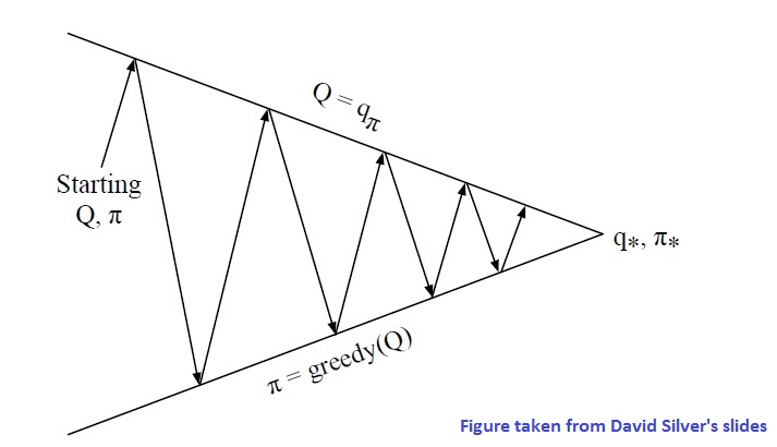
There are two points that need to be fixed in this setup:

instead of using Monte-carlo or TD methods for state-value function estimation, use them to estimate action-value function. Knowing action-value function $Q(s,a)$ allows to readily choose greedy action for a given state as in $\pi(s) = arg\max\limits_{a\in A} Q(s,a)$ .
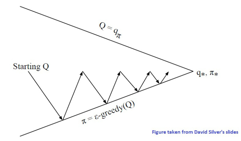
by acting greedily on the value function that is derived empirically (rather than full knowledge of dynamics), there is a chance some state or action has not been tried enough, and a potential reward is ignored. This brings the key idea of exploration. So, in deriving the new policy, we act greedily on the obtained value function with a certain probability, but also take a random action with some $\varepsilon$ probability. This is called $\varepsilon$ -greedy exploration.Thus, a new policy is derived as follows:
$\pi(a|s) = \begin{cases} \frac{\varepsilon}{m} + 1 - \varepsilon & \mbox{ if } a = arg\max\limits_{a\in A} Q(s,a) \\ \frac{\varepsilon}{m} & \mbox{ otherwise }\end{cases}$

Then, to strike a balance between eventually converging to the optimal action-value function and exploration (GLIE idea), we could make $\varepsilon$ decrease with time. This allows for exploring many states in the beginning, but eventually converging to the optimal policy.

For example, GLIE Monte-Carlo control algorithm is as follows:

Initialize $Q(s,a)$ arbitrarily
Start off with an arbitrary policy $\pi$
Sample the policy for an episode
For each state $S_t$ and action $A_t$ in the episode,
$\begin{aligned}N(S_t,A_t) & \leftarrow N(S_t, A_t) + 1 \\ Q(S_t, A_t) & \leftarrow Q(S_t,A_t) + \frac{1}{N(S_t,A_t)}\left(G_t - Q(S_t, A_t)\right)\end{aligned}$
Improve policy as follows:
$\begin{aligned}\varepsilon & \leftarrow \frac{1}{k} \\ \pi & \leftarrow \varepsilon\mbox{-greedy}(Q)\end{aligned}$
Iterate

Note that in the above, we did not wait till the convergence of the value function over several episodes for each policy before improving the policy. We modify the policy after each episode. This is typical (more efficient??) in practice. The following figures illustrates this note:

Next improvement idea is the TD idea from model-free prediction. Here, we update $Q(S_t, A_t)$ every time-step (rather than waiting till the end of the episode) using the estimated return from the Bellman equation. The algorithm gets modified as follows:

Initialize $Q(s,a)$ arbitrarily
For current state $S$ of system, take action $A$ using $\varepsilon$ -greedy policy based on $Q(s,a)$
Observe reward $R$ and subsequent state $S'$ from environment.
Choose action $A'$ (do not take action yet) based on the same policy ( $\varepsilon$ -greedy policy based on the same $Q(s,a)$ function).
Refine $Q(s,a)$ function for $s=S$ and $a=A$ as $Q(S,A)\leftarrow Q(S,A) + \alpha\left(R+\gamma Q(S',A')-Q(S,A)\right)$
Iterate the steps by taking $A'$ in state $S'$

The above algorithm is called Sarsa because of occurrence of letters $S,A,R,S',A'$ in the update of $Q(S,A)$ .

Then, similar to $n$ -step TD algorithm in model-free prediction, there is $n$ -step Sarsa in model-free control. Here, we define $n$ -step $Q$ -return as $q_t^{(n)} = R_{t+1}+\gamma R_{t+2}+\cdots+\gamma^{n-1}R_{t+n}+\gamma^n Q\left(S_{t+n}\right)$ and update as follows:

$Q\left(S_t,A_t\right)\leftarrow Q\left(S_t,A_t\right)+\alpha\left(q_t^{(n)}-Q\left(S_t,A_t\right)\right)$

And, similar to TD( $\lambda$ ) algorithm, we have Sarsa( $\lambda$ ) algorithm where we define:

$q_t^{\lambda} = (1-\lambda)\sum\limits_{n=1}^{\infty}\lambda^{n-1}q_t^{(n)}$

and we update as follows:

$Q\left(S_t,A_t\right)\leftarrow Q\left(S_t,A_t\right)+\alpha\left(q_t^{\lambda}-Q\left(S_t,A_t\right)\right)$

Value Function Approximation

Let us consider what states look like in some practical scenarios. For example, in a chess game, the state consists of layout of the board with pieces. In an Atari game, the state consists of history of a few frames of images going back from current time.

As can be seen, the number of states is enormous (in the Atari game, a state is a vector of as many dimensions as there are pixels in all frames combined). Say, each frame is 80×80 pixels, each pixel takes values 0-255 (gray scale intensities) and we need the previous four frames to represent current state adequately (position, velocity etc). This gives a state space that has a whopping $256^{80\times80\times 4}$ .

So, if we apply the RL learning algorithms directly, it is impractical to arrive at $Q$ function for all possible states (and actions) as the same state may not be seen enough number of times to be able to learn the $Q$ -value.

Further, two states may be similar mostly, but differing in some insignificant ways. For example, in a chess game, the position of a certain piece may be irrelevant given the current set up of the game. Inherently, $Q$ -values may be dependent on certain features in the states.

To make reinforcement learning practical, we use function approximators to represent the $Q$ -values for a given state and action. A function approximator is a function that approximates a target function. It is parameterized by a vector $\mathbf{w}$ such that for a certain value of $\mathbf{w}$ it becomes a close enough approximation of a target function. (Close enough approximation could mean small $L^2$ distance between the approximator and the target function)

In prediction for a given policy $\pi$ , the target function is $Q_{\pi}(S, a)$ . And, we come up with a function approximator $\hat{Q}_{\pi}(S,a,\mathbf{w})$ . The goal is to find $\mathbf{w}$ such that the objective (or cost) function $\left\lVert Q_{\pi}(S,a) - \hat{Q}_{\pi}(S,a,\mathbf{w})\right\rVert_{L^2}^2 = \mathbb{E}_{\pi}\left[\left(Q_{\pi}(S,a) - \hat{Q}_{\pi}(S,a,\mathbf{w})\right)^2\right]$ is minimized.

Assuming we know $Q_{\pi}(S,a)$ (as in supervised learning), we can apply stochastic gradient descent (SGD) to determine $\mathbf{w}$ . SGD samples (randomly chooses) the states and actions to determine the gradient. (Observe that the objective function involves summing over all the states and actions) By applying SGD with mini-batch size of just one sample (online learning??), we have that in each step of SGD, we adjust the weights with $\Delta \mathbf{w} = \alpha\left(Q_{\pi}(S,a) - \hat{Q}_{\pi}(S,a,\mathbf{w})\right){\triangledown}_{\mathbf{w}} \hat{Q}_{\pi}(S,a,\mathbf{w})$ .

In the above, we made one incorrect assumption, which is that we know $Q_{\pi}(S,a)$ . But, unlike supervised learning, we do not know the target function in reinforcement learning. In reinforcement learning, we use “presumed” targets:

In the Monte-carlo method, we use $G_t$ to get $\Delta \mathbf{w} = \alpha\left(G_t - \hat{Q}_{\pi}(S,a,\mathbf{w})\right){\triangledown}_{\mathbf{w}} \hat{Q}_{\pi}(S,a,\mathbf{w})$
In TD( $0$ ) method, we use TD target $R_{t+1}+\gamma\hat{Q}\left(S_{t+1},a,\mathbf{w}\right)$ to get $\Delta\mathbf{w} = \alpha\left(R_{t+1}+\gamma\hat{Q}\left(S_{t+1},a,\mathbf{w}\right) - \hat{Q}_{\pi}(S,a,\mathbf{w})\right){\triangledown}_{\mathbf{w}} \hat{Q}_{\pi}(S,a,\mathbf{w})$
In TD( $\lambda$ ) method, we use TD target $G_t^{\lambda}$ to get $\Delta\mathbf{w} = \alpha\left(G_t^{\lambda} - \hat{Q}_{\pi}(S,a,\mathbf{w})\right){\triangledown}_{\mathbf{w}} \hat{Q}_{\pi}(S,a,\mathbf{w})$

(The presumed targets in TD methods are also dependent on $\mathbf{w}$ . Shouldn’t gradient calculation consider the target to be function of $\mathbf{w}$ ? This is a subtle point, and fixed $Q$ -targets (see below) treat the targets as fixed.)

In practice, say, we have the following sequence of state-action pairs in a realization of the policy: $(S_1, a_1), (S_2,a_2), \cdots, (S_{T-1}, a_{T-1})$ .

In each step, we update $\Delta\mathbf{w}$ using one of the presumed targets using that one state-action pair. Recall, we do SGD with one sample of state-action pairs.

Does the stochastic gradient descent work when using presumed targets and highly correlated input state sequences? There are convergence issues that are addressed with batch method techniques like experience replay.

Example function approximators

An example type of function approximator is a linear function approximator. Here, if for each state-action pair $(S,a)$ , we are able to identify as set of features $\mathbf{x}_1(S,a), \mathbf{x}_2(S,a),\cdots, \mathbf{x}_n(S,a)$ to form a feature vector

$\mathbf{x}(S,a) = \begin{bmatrix} \mathbf{x}_1(S,a)\\ \mathbf{x}_2(S,a)\\ \vdots \\ \mathbf{x}_n(S,a)\end{bmatrix}$

then, we have a linear function approximator:

$\hat{Q}_{\pi}(S,a,\mathbf{w}) = \mathbf{x}(S,a)^T\mathbf{w}=\sum\limits_{j=1}^n \mathbf{x}_j(S,a)\mathbf{w}$

Another example type of function approximator is a deep neural network. A deep neural network is a non-linear function approximator. Deep Neural Networks have proven highly successful in feature extraction in images. In the context of reinforcement learning, we are not thinking of a two phase approach where a neural network is first used to identify specific features in the $(S,a)$ pair, and then mapping the features to $Q$ -values. Rather, the neural network automatically maps the states and action pairs to $Q$ -values, with its internal layers capturing any relevant features.

When we employ neural networks, we typically use a mini-batch of samples for SGD. We also employ the techniques of experience replay and fixed $Q$ -targets for better convergence.

$Q$ -learning is an off-policy variant of SARSA algorithm. Neural networks built to do $Q$ -learning are called Deep Q Networks (DQN).

With a DQN outputting $\hat{Q}(S,a,\mathbf{w})$ , we follow an algorithm along the lines:

Take action $a_t$ according to $\varepsilon$ -greedy policy derived from the neural network output
Store the tuple $\left(S_t, a_t, R_{t+1}, S_{t+1}\right)$ in a replay memory $D$
Sample random mini-batch of tuples from the replay memory (experience replay)
Compute presumed targets with respect to fixed parameters $\mathbf{w}^-$ (fixed $Q$ -targets)
Minimize the objective function:
$\mathbb{E}_{\left(S,a,R,S'\right) \in D}\left[\left(R+\gamma\max\limits_{a'} \hat{Q}\left(S',a',\mathbf{w}^-\right)-\hat{Q}\left(S,a,\mathbf{w}\right)\right)^2\right]$
Do this by applying SGD on the mini-batch obtained from $D$ .
Iterate

In the above, we use $\max$ in the objective function, which is different from what we saw in the SARSA algorithm. The $\max$ comes from the update step of $Q$ -learning algorithm itself, namely $Q(S,A)\leftarrow Q(S,A) + \alpha\left(R+\gamma \max\limits_{A'}Q(S',A')-Q(S,A)\right)$ .

Observe that two actions need to be chosen in the algorithms (both SARSA and $Q$ -learning) in each update step: (1) the action $A$ used to determine which state-action pairs to update $Q$ -values for (2) the action $A'$ for calculation of $Q$ -value for next state. In both SARSA and $Q$ -learning, $\varepsilon$ -greedy policy chooses actions for (1) to allow enough exploration of state-action space. Convergence of algorithms is guaranteed theoretically (??) provided algorithms do exploration, which is why they employ $\varepsilon$ -greedy, rather than greedy, for (1). The difference between SARSA and $Q$ -learning comes in (2). SARSA is an on-policy algorithm, which means it uses the same $\varepsilon$ -greedy policy for choosing action in (2). $Q$ -learning is an off-policy algorithm, which means it chooses actions for (2) differently from how it chooses actions for (1). $Q$ -learning chooses actions for (2) using $\max$ (greedy, as opposed to $\varepsilon$ -greedy) operation. $Q$ -learning converges faster(This is my guess. Is this correct?) than SARSA because it chooses action greedily in (2) in estimating $Q$ -value on next state. Such estimation is a better (??) approximation to $Q^*$ -value than an estimate obtained by choosing an action $\varepsilon$ -greedily.

Policy gradients

In the above algorithms, we first determine the $Q^*(s,a)$ (optimal $Q$ ) function. We then come up with a policy that acts $\varepsilon$ -greedy on this policy.

In algorithms based on policy gradients, we bypass the optimal value function and aim to get to an optimal policy directly.

One primary advantage of policy gradient based algorithms over value-function based algorithms is in the scenarios with continuous action spaces or many many (high-dimensional) discrete actions. When we have continuous action space, determining the maximum of $Q^*(s,a)$ function over all possible actions $a$ is impractical. On the other hand, policy gradient approaches directly determine the optimum action for a given state.

In policy gradient approach, we parameterize a policy using parameters $\theta$ . And, we need an objective function to determine how good our parameterized policy is. Example objective functions are:

Average value objection function: $J_{avV}(\theta) = \sum\limits_s d_{\pi_{\theta}}(s)V_{\pi_{\theta}}(s)$
Average reward per time-step objective function: $J_{avR}(\theta) = \sum\limits_s d_{\pi_{\theta}}(s)\sum\limits_{a}\pi_{\theta}(s,a)R_{s,a}$ .

In the above, $\pi_{\theta}$ is the policy, $d_{\pi_{\theta}}(s)$ is the stationary probability of state $s$ of Markov chain for policy $\pi_{\theta}$ , $V_{\pi_{\theta}}(s)$ is the value function, and $R_{s,a}$ is the reward obtained in state $s$ when action $a$ is taken.

An optimal policy is one with the highest value of objective function. To determine $\theta$ that maximizes the objective function, we use the stochastic gradient ascent algorithm. For the stochastic gradient descent algorithm, we first need to determine the gradients of the objective function.

Assuming average reward per time-step objective function, that is $J(\theta) = \sum\limits_s d(s)\sum\limits_{a}\pi_{\theta}(s,a)R_{s,a}$ , we have:

$\begin{aligned} \nabla_{\theta} J(\theta) &= \sum\limits_s d(s) \sum\limits_{a}\nabla_{\theta}\pi_{\theta}(s,a)R_{s,a} \\ &= \sum\limits_s d(s) \sum\limits_{a}\pi_{\theta}(s,a)\nabla_{\theta}\log\pi_{\theta}(s,a)R_{s,a} \\ &= \mathbb{E}_{\pi_{\theta}}\left[\nabla_{\theta}\log\pi_{\theta}(s,a)r\right]\end{aligned}$

In deriving the above, we used the following fact(?):

$\begin{aligned}\nabla_{\theta}\pi_{\theta}(s,a) &= \pi_{\theta}(s,a)\frac{\nabla_{\theta}\pi_{\theta}(s,a)}{\pi_{\theta}(s,a)} \\ &= \pi_{\theta}(s,a)\nabla_{\theta}\log\pi_{\theta}(s,a)\end{aligned}$

The expectation shown above is across all states and actions. The quantity $\nabla_{\theta}\log\pi_{\theta}(s,a)$ whose expectation is taken is called the score function.

A policy gradient theorem generalizes the above to multi-step scenarios as follows:

$\nabla_{\theta} J(\theta) = \mathbb{E}_{\pi_{\theta}}\left[\nabla_{\theta}\log\pi_{\theta}(s,a)Q_{\pi_{\theta}}(s,a)\right]$

An algorithm called Monte-Carlo policy gradient or REINFORCE can be used for episodic(only?) scenarios. The algorithm goes through episodes, and updates the policy by sampling the expectation (stochastic gradient ascent philosophy where rather than averaging across all states and actions, we consider one or a mini-batch of state-action pair(s)) and sampling the $Q_{\pi_{\theta}}(s,a)$ (Monte-Carlo philosophy where rather than computing $Q_{\pi_{\theta}}(s,a)$ from a model, we empirically estimate it by observing rewards(?) from episodes).

The algorithm is as follows:

Initialize $\theta$ arbitrarily.
Iterate through several(?) episodes where action in state is determined by policy .
1. Iterate through timesteps from through
  1. Update $\theta$ as $\theta = \theta + \eta\nabla_{\theta}\log\pi_{\theta}\left(s_t,a_t\right)q_t$ , where $q_t$ is a unbiased(?) sample of $Q_{\pi_{\theta}}\left(s_t,a_t\right)$

Actor-critic methods

Monte-carlo method involves a high variance on $Q_{\pi_{\theta}}(s,a)$ , since we are just using the sample $q_t$ (?). To alleviate this disadvantage, we have the Actor-critic methods which combine value-function and policy-gradient methods.

In the Actor-critic methods, there is a critic that approximates (and updates) the $Q_{\pi_{\theta}}(s,a)$ as $Q_w(s,a)$ using parameters $w$ and there is an actor that updates the policy using parameters $\theta$ .

Thus, in actor-critic methods, we use an approximate policy gradient namely

$\nabla_{\theta} J(\theta) \approx \mathbb{E}_{\pi_{\theta}}\left[\nabla_{\theta}\log\pi_{\theta}(s,a)Q_w(s,a)\right]$

We can estimate and update $Q_w(s,a)$ using the value-function based methods that we have seen earlier. Note that, we are not determining the optimal $Q(s,a)$ , but we are just determining the $Q_{\pi_{\theta}}(s,a)$ for the policy $\pi_{\theta}$ , albeit a changing policy.

Here, we give a simple actor-critic algorithm where in $Q_w(s,a) = \phi(s,a)^Tw$ is a linear function approximator that critic uses to approximate $Q_{\pi_{\theta}}(s,a)$ .

The algorithm is as follows:

Initialize $\theta$ arbitrarily. Let the initial state be called $s$ .
Sample action $a$ for state $s$ according to policy $\pi_{\theta}$
Iterate
1. Take action $a$
2. Observe reward $r = R_{s,a}$ , and next state $s'$
3. Sample action $a'$ for state $s'$ according to policy $\pi_{\theta}$
4. $\delta = r + \gamma Q_w(s',a') - Q_w(s,a)$
5. $\theta = \theta + \alpha\nabla_{\theta}\log\pi_{\theta}(s,a)Q_w(s,a)$
6. $w = w + \beta\delta\phi(s,a)$
7. $a = a', s = s'$

A variant of the above algorithm uses advantage function $A_{\pi_{\theta}} = Q_{\pi_{\theta}}(s,a) - V_{\pi_{\theta}}(s)$ , which results in (?) $\nabla_{\theta} J(\theta) = \mathbb{E}_{\pi_{\theta}}\left[\nabla_{\theta}\log\pi_{\theta}(s,a)A_{\pi_{\theta}}(s,a)\right]$ .

Two policy gradient methods are described here and here.